Introduction
Excel is a powerful tool for organizing, analyzing, and presenting data. But what truly sets it apart from other similar programs is its ability to perform complex calculations through the use of formulas. In this article, we’ll explore some of the most important and commonly used formulas in Excel and show you how to use them to transform your spreadsheets into dynamic, data-driven tools.
Basic Arithmetic Formulas
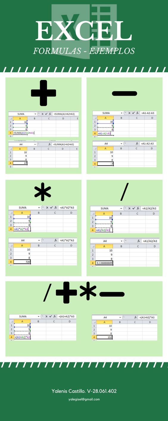
Excel allows you to perform simple arithmetic operations such as addition, subtraction, multiplication, and division using the basic operators: +, -, *, and /. For example, to add the values in cells A1 and B1, you would enter the formula “=A1+B1” into a blank cell. The result of the calculation will be displayed in that cell.
SUM and AVERAGE Formulas
The SUM and AVERAGE formulas are two of the most frequently used formulas in Excel. The SUM formula allows you to add up a range of cells, while the AVERAGE formula calculates the average of a range of cells. For example, to find the sum of the values in cells A1 through A10, you would enter the formula “=SUM(A1:A10)” into a blank cell. To find the average of those same cells, you would use the formula “=AVERAGE(A1:A10)”.
IF Formulas
The IF formula is one of the most powerful formulas in Excel. It allows you to perform conditional calculations, meaning you can specify that a certain result should be displayed only if a certain condition is met. For example, to display “Pass” if the value in cell A1 is greater than 50 and “Fail” if it is less than or equal to 50, you would enter the formula “=IF(A1>50, “Pass”, “Fail”)” into a blank cell.
VLOOKUP Formulas
The VLOOKUP formula allows you to search for a specific value in a table and return a corresponding value from another column in the same row. For example, if you have a table with product names and prices, you could use a VLOOKUP formula to search for a specific product and return its price. This is especially useful for large tables of data where manual searching would be time-consuming and error-prone.
HLOOKUP Formulas
The HLOOKUP formula is similar to the VLOOKUP formula, but it searches for a value in the first row of a table instead of the first column. This allows you to perform horizontal lookups, which can be useful in certain cases where you need to search for a value across multiple columns.
INDEX and MATCH Formulas
The INDEX and MATCH formulas are a powerful combination that allow you to search for a value in a table and return a corresponding value from a different column. The MATCH formula is used to search for a value, while the INDEX formula is used to return the corresponding value. This combination is more flexible than the VLOOKUP and HLOOKUP formulas and can be used in a wider range of situations.
You might find these FREE courses useful:
- Using Advanced Formulas and Functions in Excel
- Using Basic Formulas and Functions in Microsoft Excel
- Excel Basics for Data Analysis
- Work Smarter with Microsoft Excel
Text Formulas
Excel also includes a variety of formulas for working with text. For example, the CONCATENATE formula allows you to join two or more text strings into a single string. The LEFT, RIGHT, and MID formulas allow you to extract specific characters from a text string, while the LEN formula returns the number of characters.
Conclusion
Excel formulas are a powerful tool for organizing, analyzing, and presenting data. Whether you’re working with basic arithmetic operations, conditional calculations, or more advanced functions,


